In response to the conundrum: it is better to think in terms of asynchrony.
The behaviour of the North and South hemispheres, would suggest that the nature of the climate system is analogous to a seesaw, with each hemisphere taking turns to drive the system. (Note; this change is in response to millennial-scale climate variability). To revisit, it has been acknowledged that iceberg discharges into the North Atlantic caused a disruption of the Atlantic meridional overturning circulation (AMOC), causing a cooling of northern hemisphere and warming of Antarctica (Rahmstorf,2002) . This one of two schools of thought on mechanisms of millennial-scale climate variability (externally forced climate change and internal ice-sheet dynamics, the former is what we will focus on in this post).
There has been a substantial volume of literature written on the subject of ‘seesaw’. Broecker (1998) coined the term; in light of the thesis that abrupt cooling in the North Atlantic would leave a distinctive signal in the South Atlantic; with changes in the north and south occurring in synchrony. Stocker (1998), also suggested an oceanic seesaw whereby changes are driven by high-latitudinal or near-equatorial changes or, a combination of both.
However, the original bipolar seesaw concept has been subject to scrutiny (Stocker and Johnsen, 2003). Firstly, the original bipolar seesaw model suggests that changes in north and south occurred in phase. This is out of course divergence from records in Antarctica and Greenland and also for the fact that this requires very fast heat transmission in the oceans (which as we now, is difficult given the thermal inertia of the oceans). It also must be noted that the bipolar seesaw must not be used as an all-encompassing term to describe all climate changes where interhemispheric connections exist; it is a term to describe responses to millennial-scale climatic changes.
Stocker and Johnsen (2003) postulate a ‘thermal bipolar seesaw’, by coupling a heat reservoir to the original bipolar seesaw model (Figure 1). They apply this conceptual model to GRIP and Byrd data (shown in last post) and highlight that correlation can be achieved on a timescale of 1000-1500 years.

Figure 1. Schematic model of the thermal bipolar seesaw. The bipolar seesaw is joined to a heat reservoir (potentially the Southern Ocean). Double arrow indicates that heat exchange with the reservoir is taken to be diffuse.
Source: Stocker and Johnsen (2003).
In short, the model suggests that the asymmetric response of both hemispheres can be explained by a bipolar seesaw mechanism in which changes in the strength of AMOC can contribute to changes in interhemispheric heat transport.
However, what is the likely to drive changes in this seesaw?
Due to large volume and thermal inertia, it is likely the deep ocean is likely (Rahmstorf, 2002). There is however, an additional complexity; the notion of thresholds in north-atlantic deepwater system. Based on Greenland and the Iberian margin, Rahmstorf (2002) shows there are 3 modes; stadial, interstadial and Heinrich mode (Figure 2). In the interstadial mode (warm, modern and interglacial), North Atlantic Deep Water (NADW) forms in the Nordic seas. In the stadial mode; it forms in the subpolar open North Atlantic (leading to a cold, glacial D-O stadial) and in the Heinrich mode, NADW formation all but ceased and waters of Antarctic origin filled deep Atlantic basin.
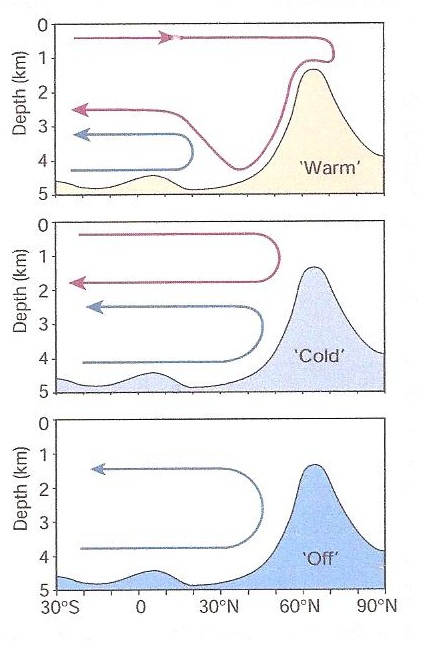
Figure 2: Schematic version of the three modes (‘warm’, ‘cold’ and ‘off’) of ocean circulation as observed during different times of the last glacial period. Shown is the section along the Atlantic, with NADW highlighted by the red line and AABW by the blue line.
Source: Rahmstorf (2002).
There is an enormous difficulty in quantifying the risk of abrupt changes in deep-water circulation. This is due to the possibility of a NADW bifurcation, coupled with the fact that we do not know the state of the current climate system with regards to the threshold (a point I made all the way back in post 2).
These 3 modes of deep water circulation and the bipolar seesaw mechanism highlight the non-linearity and uncertainty in our understanding of millennial-scale climate variability. This in turn, has significant implications when trying to understand and predict the impacts of climate change.
Hi Jas - Having read some of your posts on the mechanics of our oceans it is clear to me that there is not only enormous complexity involved but also a great uncertainty in terms of quantitative contributions from academics.
ReplyDeleteWith the Integrated Earth Systems approach a key paradigm in modern Earth Science, to what extent do you feel the oceans are the major cause of both a lack of certainly and significant progress in this regard, and what is being done to improve our approaches to gaining more accurate quantitative perspectives of ocean mechanics?
Hi Joe- many thanks for the post. If one drew a spectrum of climate change, integrating scales of change (i.e. from 10-5, 10-4, 10,-3, 10-2, 10-1 and present) you would find that you have Milankovitch parameters (10-5 to 10-4) followed by millenial-scale changes (H events, D/O cycles at 10-4) you would find a gap between 1000s and 100s of years (NB 10-1- solar cycles, NAO and ENSO oscillation). Here, oceans could be a major cause of this uncertainty but as could be all the other parameters accounted by the earth systems approach. Furthermore, if one looks at modelling approaches to response to change in the climate system, you can argue oceans are a leading cause due to the discovery of non-linear changes (e.g. thermohaline circulation) and bifurcations (e.g. bipolar seesaw concept as above). However, I would argue that in the earth systems approach, the major cause of uncertainty and lack of progress is the simple fact that all the earth system parameters respond on different time-scales of change and in different ways (e.g. linear, non-linear, muted and threshold response) and this signal can be amplified further by feedbacks. However, "noise" in the climate system (or unknown as I would call it) complicates our ability to attribute these signals to certain parameters or feedback progresses. Thus, this leaves a problem of attribution which is a key barrier to significant progress.
ReplyDeleteRegarding the second question, a body of literature has arisen which has sought to refute the narrow 'trap' in understanding the North Atlantic thermohaline circulation which is to focus only on freshwater and salinity content(More info can be found in blog post 2). Drawing on ocean physics, this approach has sought to emphasise the role of tidal motions and wind fields. Drawing on geophysical fluid dynamics, this approach has also emphasised that whilst water sinks and fills the deep ocean in the North Atlantic (as observed with North Atlantic deep water), the rest of the circulation moves in a 3D fashion. Thus, it emphasises the importance of being critical in our use of terms such as 'global ocean conveyor belt'. Whilst quantification is still afar, this literature has sought to set the pre-occupation of quantifying freshwater hysterisis of the North Atlantic thermohaline circulation in the context of global ocean mechanics.
I would recommend the following papers:
- Wunsch, C. (2002) 'What is the thermohaline circulation?', Science, 298, 1179-1180
Lozier, S. M. et al (2010) 'Deconstructing the conveyor belt', Science, 328, 1507, 1511